Cart Pole Dynamics Simulation
The goal of this project was to use material learned in the CSCI 6150 class to simulate a Cart Pole system. The most heavily referenced materials for this project were the Underactuated Robotics course materials from MIT and the various papers of Mattew Peter Kelly, though some additional materials were used.
Seriously, I learned most of this from Mattew Peter Kelly, check out his website it is awesome!
The code for this project is located at https://github.com/piepieninja/Cart-Pole-Dynamics.
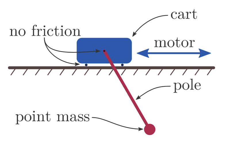
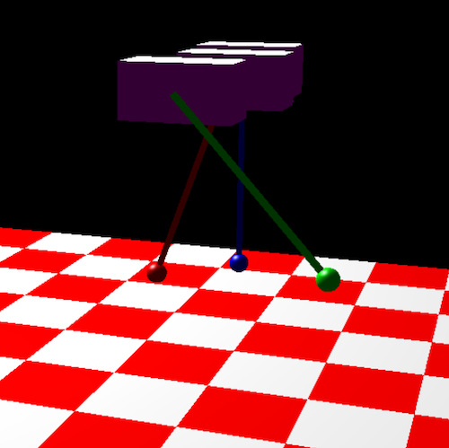
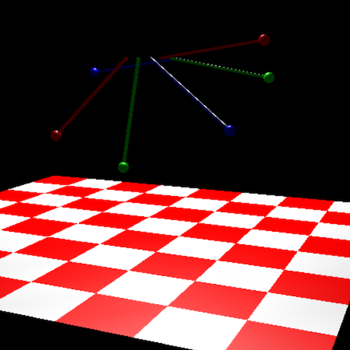
The Cart Pole system consists of a Cart, which is free to roll in the x directions, and a pendulum which is free to rotate around the center of the cart. The pole and the cart transfer energy between one another, with the total energy of the system being constant. Only friction and damping due to wind resistance would remove energy from the system. Once should also consider that the Cart and the Pole are exerting forces of varying magnitudes on one another over time. This is was allows the system to be described as a set of second order equations. A video can be seen below:
Dynamics of the Cart Pole
A Balance of forces can be see on the Cart Pole in Figure 2. This balance of forces is what is used to generate the equations which govern the Cart Pole.
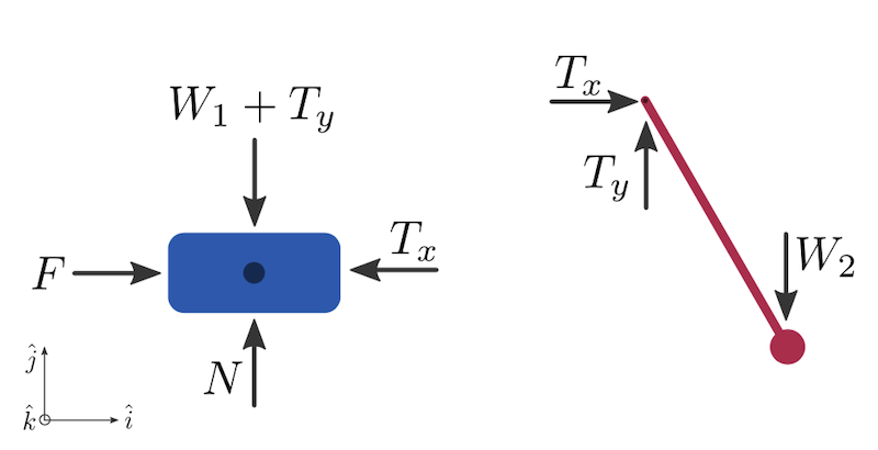
From these free body diagrams, we can generate 3 equations (the force balance on the cart, the balance on the pole, and the balance around the pivot):
\[\begin{equation} (F - T) \hat{i} + (N - W_1 - T_y) \hat{j} = m_1 \ddot{p_1} \end{equation}\] \[\begin{equation} (T_x) \hat{i} (T_y - W_2 ) \hat{j} = m_2 \ddot{p_2} \end{equation}\] \[\begin{equation} (T_x) \hat{i} (T_y - W_2 ) \hat{j} = m_2 \ddot{p_2} \end{equation}\]In the end, these equations give us the following second order linear system to describe the cart pole:
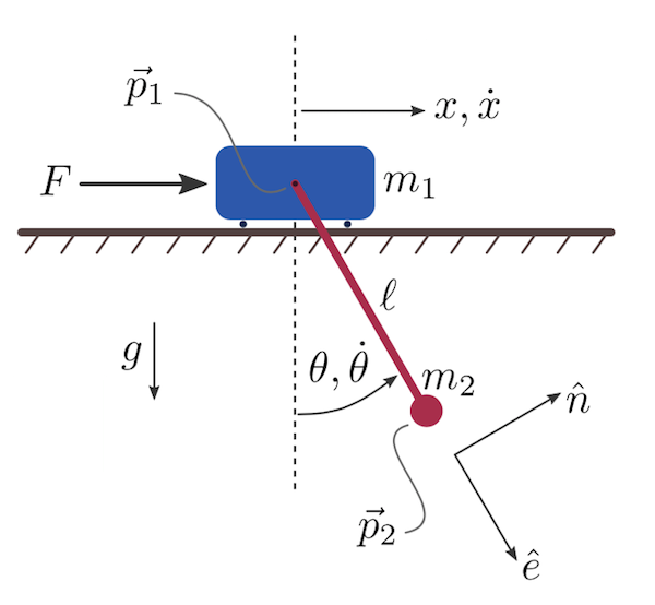
\[\begin{equation} \label{eq:4} \begin{bmatrix} \cos \theta & l \\ m_1 + m_2 & m_2 l \cos \theta \end{bmatrix} \begin{bmatrix} \ddot{x} \\ \ddot{\theta} \end{bmatrix} = \begin{bmatrix} - g \sin \theta \\ F + m_2 l \dot{\theta}^2 \sin \theta \end{bmatrix} \end{equation}\]For the purpose of this project I transform this system back into two functions. This system can be viewed as \(A x = b\), so simply \(x = A^{-1} b\) will give us a solution. Then, we can solve for the second derivatives. Doing this yields the following two equations:
\[\begin{equation} \label{eq:5} \ddot{x} = \frac{-g \sin \theta m_2 l \cos \theta + (-l)(F + m_2 l \dot{\theta}^2 \sin \theta) }{ (\cos \theta)^2 m_2 l - l(m_1 + m_2) } \end{equation}\] \[\begin{equation} \label{eq:6} \ddot{\theta} = \frac{-(m_1 + m_2)(-g \sin \theta) + \cos \theta (F + m_2 l \dot{\theta}^2 \sin \theta) }{ (\cos \theta)^2 m_2 l - l(m_1 + m_2) } \end{equation}\]Methods Used and Implementation
In general, this was formulated as an Initial Value Problem (IVP), solved accordingly, and then simulated using OpenGL.
Formulation as a System of ODEs
This problem was solved using techniques found in chapter 11 of Numerical mathematics and Computing. First, The variables are substituted and make into a system of first order equations.
\[X = \begin{bmatrix} x_1 = x \\ x_2 = \dot{x} \\ x_3 = \theta \\ x_4 = \dot{\theta} \end{bmatrix} , \hspace{2mm} X(0) = \begin{bmatrix} x_1 = 0 \\ x_2 = 0 \\ x_3 = \pi / 4 \\ x_4 = 0 \end{bmatrix}\]Then, we note that we can describe the state vector \(X\)’s derivative vector \(\dot{X}\), which is what we can use to solve an IVP with the system. Note that this is where we want to jump back to the separated equations 5 and 6 in part 2. These equations will not take the forms:
\[\begin{equation} F(x_3, x_4) = \frac{-g \sin x_3 m_2 l \cos x_3 + (-l)(F + m_2 l x_4^2 \sin x_3) }{ (\cos x_3)^2 m_2 l - l(m_1 + m_2) } \end{equation}\]and …
\[\begin{equation} G(x_3, x_4) = \frac{-(m_1 + m_2)(-g \sin x_3) + \cos x_3 (F + m_2 l \dot{x_4}^2 \sin x_3) }{ (\cos x_3)^2 m_2 l - l(m_1 + m_2) } \end{equation}\]Then we form the derivative vector \(\dot{X}\):
\[\dot{X} = \begin{bmatrix} \dot{x_1} \\ \dot{x_2} \\ \dot{x_3} \\ \dot{x_4} \end{bmatrix} = \begin{bmatrix} x_2 \\ F(x_3, x_4) \\ x_4 \\ G(x_3, x_4) \end{bmatrix}\]This then allows us to form the simplest IVP, using Euler’s method with a stepsize \(h\):
\[\begin{equation} \label{eq:9} X(t+1) = X(t) + h \cdot \dot{X}(X(t),t) \end{equation}\]This also allows for a Modified Euler’s method with stepsize \(h\):
\(K_1 = \dot{X}(X(t),t)\) \(K_2 = \dot{X}(X(t+1) + h \cdot K_1,t+1)\)
\[\begin{equation} \label{eq:10} X(t+1) = X(t) + h \frac{K_1 + K_2}{2} \end{equation}\]And finally, this allows for an RK4 method to be used, here shown with stepsize \(h\):
\(K_1 = \dot{X}(X(t),t)\) \(K_2 = \dot{X}(X(t)+ \frac{h}{2} K_1,t + \frac{h}{2})\) \(K_3 = \dot{X}(X(t)+ \frac{h}{2} K_2,t + \frac{h}{2})\) \(K_4 = \dot{X}(X(t)+ h K_3,t + h)\)
\[\begin{equation} X(t+1) = X(t) + h \frac{K_1 + 2K_2 + 2K_3 + K_4}{6} \end{equation}\]These three methods, Euler, Modified Euler, and RK4 are Implemented in this project. These are
methods in the Cart Pole Object within the sim_cartpole.cpp file. Additionally,
the Euler method is implemented for some simple pendulums within the sim_pendulum.cpp
file.
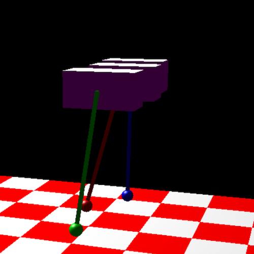
OpenGL and Rendering
This simulation uses OpenGL and the OpenGL Utilities. These libraries are used to draw primitive poles, boxes, and spheres. Various matrix transformations, which can occur with OpenGL provided functions, are used to shift the simulated objects across the render area. Additionally, the setup and outline of the c++ code used is heavily based on the OpenGLUT examples from Ray Toal’s class.
The readme at the root of this project should provide adequate instructions on how to run the program. When the program starts you can use the arrow keys to rotate your view and see more of the simulation.
Results and Future Work
Simulation Results
Overall the results are quite nice. The standard Euler method works well and transfers energy and momentum throughout the system as I would expect. However, it was difficult to judge if results were correct, as the cart pole is a chaotic system. The changes in types of numerical methods would make the chaotic nature of the system apparent after only a few iterations, and that makes it hard to directly compare methods. Additionally, the lack of a clear closed loop solution to the cart pole makes it difficult to compare each individual result to a ground truth.
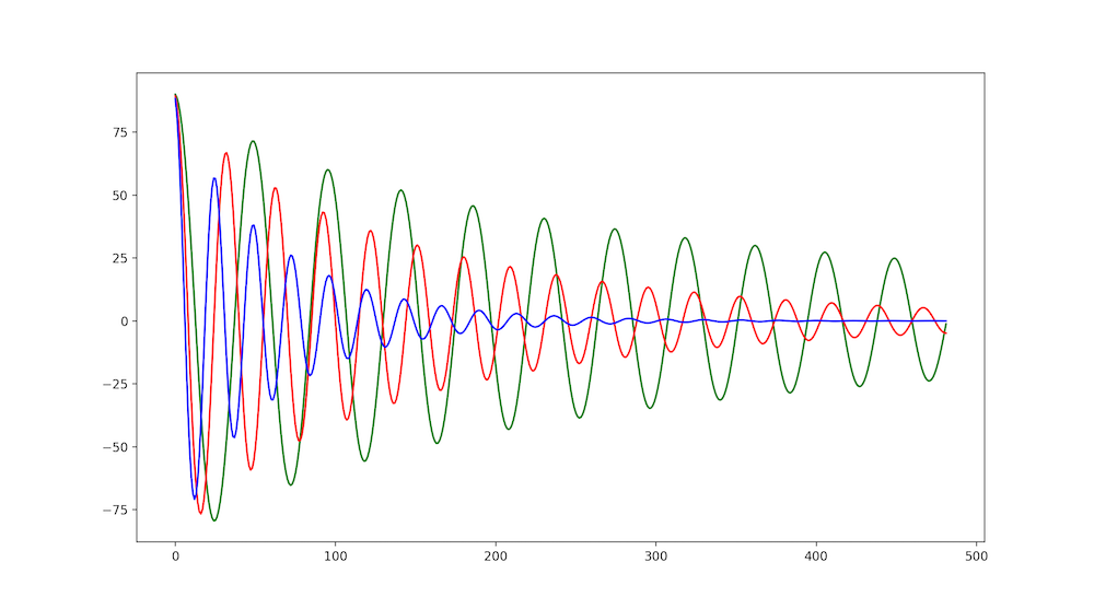
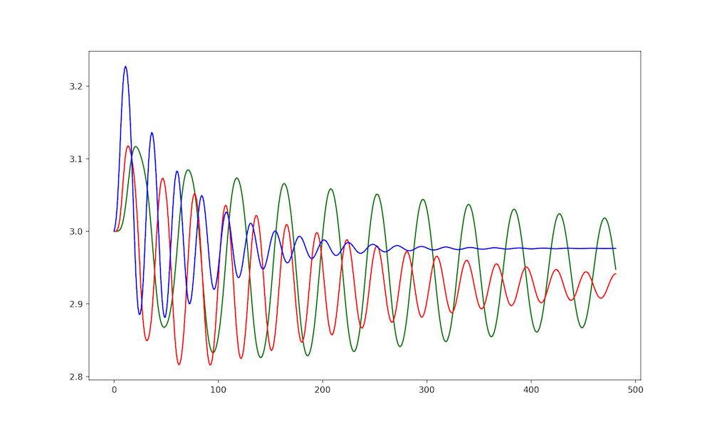
Many simulations, or models used for Trajectory Optimization, do not account for a dampening factor or friction on the cart system. I attempted to model these, which is clear in Figures 4 and 5 as the amplitude clearly decreases over time. I do not think I adequately modeled these dampening and friction forces, but as I mentioned above it is hard to tell due to the chaotic nature of the Cart Pole. I would at least expect the rate of dampening to be similar in each method, which is not something I see and leads me to believe there is some error associated to that.
It is likely that I have not modeled the nuances of friction in the system correctly, and this could be what is causing the divergent behavior with the amplitudes between methods. I assumed that I could model both friction and the damping factor as a simple \(- \mu \ddot{x}\) and \(- \mu \ddot{\theta}\), where \(mu\) is some constant coefficient. However, this is likely untrue, as friction is tied to the normal force. For example, it is commonly know that \(F_f \leq \mu F_n\) where \(\mu\) is the coefficient of friction, \(F_n\) is the normal force, and \(F_f\) is the true force of friction. This implies that the Cart Pole does not experience a constant force due to friction (which is what I am currently modeling), as the normal force generated by the pole will vary by its angle. This means that there is a separate set of component forces that are not being modeled, as the swing-up of the pole would cause the normal force \(F_n\) to vary with the state of the pole. This could explain the strange dampening of the modeled system and would need to be addressed to make the system more accurate. What could complicate this further is that the cart pole cannot shake, as the motion of the cart is constrained to the x axis. This is unrealistic in many ways. If the pole were to swing up fast enough and have a large enough mass, it is realistic to expect the cart to shake and move within the plane of the pole - not just the x axis.
Future Work
In the future I plan to derive the correct friction related equations as well as attempt to control the cart pole system with the framework I have built. Once I can formulate the system as an IVP, I will attempt to formulate it as a BVP. This is so that I can perform Trajectory Optimization so that I can control the cart pole in an upright state. The reason a BVP style solution is desired is because it can specify a starting condition and an ending condition. It’s possible that the Trajectory Optimization could be combined with a simple controller.