N View Triangulation of 3D Skew Lines

---

Overview

we expect points in the form \(P = (p_x, p_y, p_z)\) and their corresponding orientation as a unit vector \(\hat{U} = (\hat{u}_x, \hat{u}_y, \hat{u}_z)\), we expect these together in a tuple \(((p_x, p_y, p_z), (\hat{u}_x, \hat{u}_y, \hat{u}_z))_n\). This tuple comes with several (\(n\) many) tuples which all uniquely correspond with a matched set. So we have a \(\mathbb{R}^{3}\) match set \(M = \{ (P, \hat{U})_0, (P, \hat{U})_1, ... , (P, \hat{U})_n \}\) where \(n\) is the number of tuple pairs and has a one-to-one correspondence with the number of views in which the \(\mathbb{R}^{2}\) match was found. We all also get a set of \(\mathbb{R}^{3}\) matches, \(M_i\), resulting in a set which has a one-to-one correspondence with the total number of points we should have after reprojection.

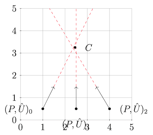
In the figure above, assume that point \(C\) is the correct real world point and has no orientation. The goal is to make a best guess at the value of \(C\) given our imperfect information.

A 3 by 3 Inversion Method

A method which finds a “midpoint” for n many views with minimal computational cost is described as follows. At this point we do not actually know the coordinates of the real point \(C\), but we will proceed to derive how to find it. First, consider the identity:

\[(m \times n) \cdot (m \times n) = || m ||^2 || n ||^2 - (m \cdot n)^2\]

Then note, we have the distance function, measuring how much a given \(((p_x, p_y, p_z), (\hat{u}_x, \hat{u}_y, \hat{u}_z))_n\) tuple (which represents a line) misses the real world target point \(C\). Note this function is calculated for each tuple.

\[D_n = \frac{||(C - P_n) \times \hat{U}_n || }{ || \hat{U}_n ||}\]

We will want to use the square of the distance (as is common in many optimization problems) to insure convex optimization and positive distance values. We also use the identity mentioned above to get our primary distance equation. Then, taking the first derivative of the distance function will give us a local minimum value by finding a \(0\) solution.

\[\begin{equation} \begin{split} D_n &= \frac{||(C - P_n) \times \hat{U}_n || }{ || \hat{U}_n ||} \\ D_n^2 &= \Big( \frac{||(C - P_n) \times \hat{U}_n || }{ || \hat{U}_n ||} \Big)^2 \\ D_n^2 &= \frac{||(C - P_n) \times \hat{U}_n ||^2 }{ || \hat{U}_n ||^2 }\\ D_n^2 &= \frac{ || C - P_n ||^2 || \hat{U}_n ||^2 - ||(C - P_n) \cdot \hat{U}_n ||^2 }{ || \hat{U}_n ||^2 }\\ D_n^2 &= || C - P_n ||^2 - \frac{ ||(C - P_n) \cdot \hat{U}_n ||^2 }{|| \hat{U}_n ||^2} \\ \frac{d D_n^2}{d C} &= 2 (C - P_n) - 2 \hat{U}_n \frac{ (C - P_n) \cdot \hat{U}_n }{ || \hat{U}_n ||^2 } \end{split} \end{equation}\]

So, we need to find a zero for the following (note that we are dealing with a vector in \(\mathbb{R}^{3}\), so \(0 = [0 , 0, 0]^T\)). The value \(m\) is the total number of \(\mathbb{R}^{3}\) match points:

\[\begin{equation} \begin{split} 0 &= \sum_{n=0}^m C - P_n - \hat{U}_n \frac{ (C - P_n) \cdot \hat{U}_n }{ || \hat{U}_n ||^2 }\\ 0 &= \sum_{n=0}^m C - P_n - \frac{ \hat{U}_n ( C \cdot \hat{U}_n ) }{ || \hat{U}_n ||^2 } + \frac{ \hat{U}_n ( P_n \cdot \hat{U}_n ) }{ || \hat{U}_n ||^2 } \\ 0 &= \sum_{n=0}^m C - P_n - \frac{ \hat{U}_n \hat{U}_n^T C }{ || \hat{U}_n ||^2 } + \frac{ \hat{U}_n \hat{U}_n^T P_n }{ || \hat{U}_n ||^2 }\\ 0 &= \sum_{n=0}^m \Big( I - \frac{ \hat{U}_n \hat{U}_n^T }{ || \hat{U}_n ||^2 } \Big) C - \Big( P_n - \frac{ \hat{U}_n \hat{U}_n^T P_n }{ || \hat{U}_n ||^2 } \Big) \end{split} \end{equation}\]

Notice this is of the form \(Ax = b\) because we now have \(0 = Ax - b\). The next thing to note is we can remove the summations and get a system that results in taking an inverse of a 3 by 3 matrix.

Notice the possible expansion:

\[\begin{equation} \begin{split} 0 &= \sum_{n=0}^m \Big( I - \frac{ \hat{U}_n \hat{U}_n^T }{ || \hat{U}_n ||^2 } \Big) C - \Big( P_n - \frac{ \hat{U}_n \hat{U}_n^T P_n }{ || \hat{U}_n ||^2 } \Big)\\ 0 &= \Bigg( \Big( I - \frac{ \hat{U}_0 \hat{U}_0^T }{ || \hat{U}_0 ||^2 } \Big) + \Big( I - \frac{ \hat{U}_1 \hat{U}_1^T }{ || \hat{U}_1 ||^2 } \Big) + \Big( I - \frac{ \hat{U}_2 \hat{U}_2^T }{ || \hat{U}_2 ||^2 } \Big) + ... \Bigg) C \\ &- \Bigg( \Big( P_0 - \frac{ \hat{U}_0 \hat{U}_0^T P_0 }{ || \hat{U}_0 ||^2 } \Big) + \Big( P_1 - \frac{ \hat{U}_1 \hat{U}_1^T P_1 }{ || \hat{U}_1 ||^2 } \Big) + ... \Bigg) \\ 0 &= (A) C - (b)\\ AC &= b \\ C &= A^{-1}b \end{split} \end{equation}\]

So, the meat of this method is to calculate the \(A\) matrix’s inverse and muplyply it by vector \(b\) to find the estimated point \(C\). succinctly, these are calcualted:

\[\begin{equation} A = \sum_{n=0}^m \Big( I - \frac{ \hat{U}_n \hat{U}_n^T }{ || \hat{U}_n ||^2 } \Big) \end{equation}\] \[\begin{equation} b = \sum_{n=0}^m \Big( P_n - \frac{ \hat{U}_n \hat{U}_n^T P_n }{ || \hat{U}_n ||^2 } \Big) \end{equation}\]

Then, because this method takes the inverse of a 3x3 matrix, we can easily write (hardcode) a constant time inversion method. This makes the method an ideal N-view triangulation method. Additionally consider that this is run on GPU, so the point estimations can occur in parallel for each matched set of points. Similar benefits could be realized running the algorithm on a multithreaded system.

This is copied from a section of my thesis. If you found this useful to your research please consider using the following bibtex:

@mastersthesis{CalebAdamsMSThesis,
  author={Caleb Ashmore Adams},
  title={High Performance Computation with Small Satellites and Small Satellite Swarms for 3D Reconstruction},
  school={The University of Georgia},
  url={http://piepieninja.github.io/research-papers/thesis.pdf},
  year=2020,
  month=may
}